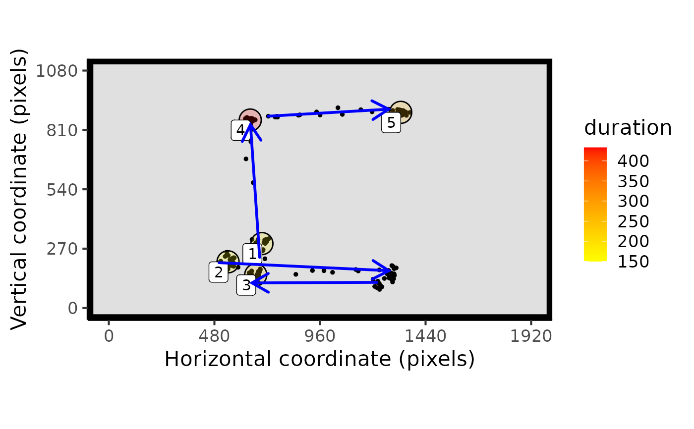
Plot raw data and fixations — spatial

A tool for visualising raw eye-data, processed fixations, and saccades. Can all three data types. Fixations can be labeled in the order they were made. Can overlay areas of interest (AOIs) and customise the resolution.

Usage

spatial_plot(
  raw_data = NULL,
  fix_data = NULL,
  sac_data = NULL,
  AOIs = NULL,
  bg_image = NULL,
  res = c(0, 1920, 0, 1080),
  flip_y = FALSE,
  show_fix_order = TRUE,
  plot_header = FALSE
)

Arguments

raw_data: data in standard raw data form (time, x, y, trial)
fix_data: data output from fixation function
sac_data: data output from saccade function
AOIs: A dataframe of areas of interest (AOIs), with one row per AOI (x, y, width_radius, height). If using circular AOIs, then the 3rd column is used for the radius and the height should be set to NA.
bg_image: The filepath of an image to be added to the plot, for example to show a screenshot of the task.
res: resolution of the display to be shown, as a vector (xmin, xmax, ymin, ymax)
flip_y: reverse the y axis coordinates (useful if origin is top of the screen)
show_fix_order: label the fixations in the order they were made
plot_header: display the header title text which explains graphical features of the plot.

Examples

#trying to draw a screenshot under a spatial plot
d_raw <- example_raw_WM
d_raw <- d_raw[d_raw$trial==10,] # take just one trial
d_fix <- fix_dispersion(d_raw)
d_sac <- VTI_saccade(d_raw)
spatial_plot(raw_data = d_raw,
             fix_data = d_fix,
             sac_data = d_sac)