9 Week 9: Unrelated-samples t-test and Power
Written by Tom Beesley & John Towse
9.1 Pre-lab work: online tutorial
Online tutorial: You must make every attempt to complete this before the lab! To access the pre-lab tutorial click here (on campus, or VPN required)
Getting ready for the lab class
Create a folder and a Project for Week 9. Click here for the instructions from Week 6 if you are unsure.
Download the Week_9.zip file and upload it into this new folder in RStudio Server. If you need them, here are the instructions from Week 2.
9.2 Data visualisation and cleaning
In this class we will be exploring some data on music preferences and social media use. In our survey we asked people to rate how much they liked various music artists out of 5. There were some “pop” artists like Beyonce and Taylor Swift, and some “rock” artists like Coldplay and Nirvana. In the data we have grouped the ratings for pop artists together, and similarly for the rock artists: each respondent therefore gets a pop_score and a rock_score. We’ve also turned these ratings into a categorial variable, which reflects whether someone liked pop more than rock (“pop-tastic”), or not (“rock-on” - either they preferred rock, or they had no preference).
The other variables relate to social media use. We have the instagram_followers and facebook_friends, which provide a (fairly crude) measure of how much someone engages with these social media platforms.
Let’s first take a look at the data on music preferences. We might think that people who like rock music are less likely to be in to pop music (and vice versa). To look at this relationship we can plot one score on the x axis and one on the y axis. Read in the data (make sure it’s called “data_w9”) and complete the
geom_jitter()code to do this (we usegeom_jitter()here because there are overlapping points).Consider the pattern of data you see. In general, do people who really like pop (high scores) like or dislike rock? Conversely, do those who like rock dislike pop? What pattern would you expect for these different relationships in preference? Talk about it with your table.
Next you can add a mapping between music_pref and colour to show our boundaries for the two levels of the categorical variable
Let’s take a look at the two social media variables. Complete the code for the two histogram plots to view the data on facebook friends and instagram followers.
You’ll see that for both variables, there are some extreme values (some people have >1000 friends and > 2000 followers). These outlier values can be problematic when we run our statistical tests, so (like last week) we probably want to control their influence by removing them. As you saw in your online tutorial, we can convert the data to z scores, and then remove z values above and below certain values.
Let’s create two “z-transform columns”. Complete the code by adding the two variable (column) names to the code. View the data_w9 object to check these have been created correctly. Like in the online tutorial, it would be a good idea to calculate some descriptive statistics for these new columns to check them (e.g.,
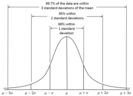
mean(),sd(),min()andmax()).We know from our lectures on the z distribution that values of greater than 2 (or less than -2) reflect around 5% of the distribution, and values greater than 3 (or less than -3) represent less than 1% of the distribution:
- Let’s consider an outlier any value that has a z of 2.5 (a conventional cutoff). Complete the filter command to remove the data where the z value is greater than 2.5 for both the z_FF column and the z_IF column. Note you only need to look at positive values: our histogram has already shown that these data are positively skewed with outliers only at the positive end (you cannot have fewer than 0 friends/followers; these are ratio scales with a true 0 value). Complete the filter command to remove the positive z values above 2.5. When completing this, note the use of the AND (&) symbol: We want to KEEP z values that are below 2.5 for both the z_FF and z_IF variables.
9.4 Power and effect size (d) calculations
We saw in last week’s lab tasks that there was a significant effect in our Stroop task data: participants were faster to say the colour names of the compatible list compared to the incompatible list (there were significant differences with the control list too). We will now use these data to calculate an effect size (Cohen’s d) for the t-statistic that we observed in that test.
Import the stroop data. It’s always a good idea to
view()it (you can do this by clicking on it in the environment) to remind yourself what it looks like.Run the code that will
filter()the data to the two conditions we are interested in (compatible and incompatible).Run the
cohens_d()code to calculate the effect size, which is reported as effsize. You can ignore any negative sign, taking note of the absolute value.So we know that this large effect size was significant with our fairly large sample of participants. What might we have expected with a much smaller sample size. Use the
pwr.t.test()function to add in the effect size (d) and an N of 20. What power would we have achieved with this sample size, to detect this large effect?Let’s say we wanted our next experiment to have an 80% chance of finding an effect at least as large as the one we found. Complete the
pwr.t.test()function to work out the minimum sample size we would need to achieve power of .8, with this effect size.Let’s say we are looking to run a new experiment in which we give people a stressful task to complete simultaneously. We will ask them to put their hands in a bucket of ice cold water while doing the Stroop task. We are unsure of what consequence this will have for our effect size, but we want to estimate the effect size that could be achieved. We decide to run 40 participants, and want to achieve a power of .90 (90% chance to find an effect at least this large). What is the minimum effect size we could hope to detect under these conditions?
9.5 Answers
When you have completed all of the lab content, you may want to check your answers with our completed version of the script for this week. Remember, looking at this script (studying/revising it) does not replace the process of working through the lab activities, trying them out for yourself, getting stuck, asking questions, finding solutions, adding your own comments, etc. Actively engaging with the material is the way to learn these analysis skills, not by looking at someone else’s completed code…
Download the answers script