Animating eyetools Data

In this article, we offer examples of how eyetools data can be used with the gganimate package. This article is code heavy as it is designed to demonstrate the capacity of gganimate in tandem with eyetools and for relatively straightforward application to one’s own data.

library(eyetools)
library(gganimate)
library(tidyverse)
library(zoo)

data <- combine_eyes(HCL) |> 
  interpolate(participant_ID = "pNum")

data_smooth <- smoother(data, span = .02, participant_ID = "pNum")

Plotting raw data with lag

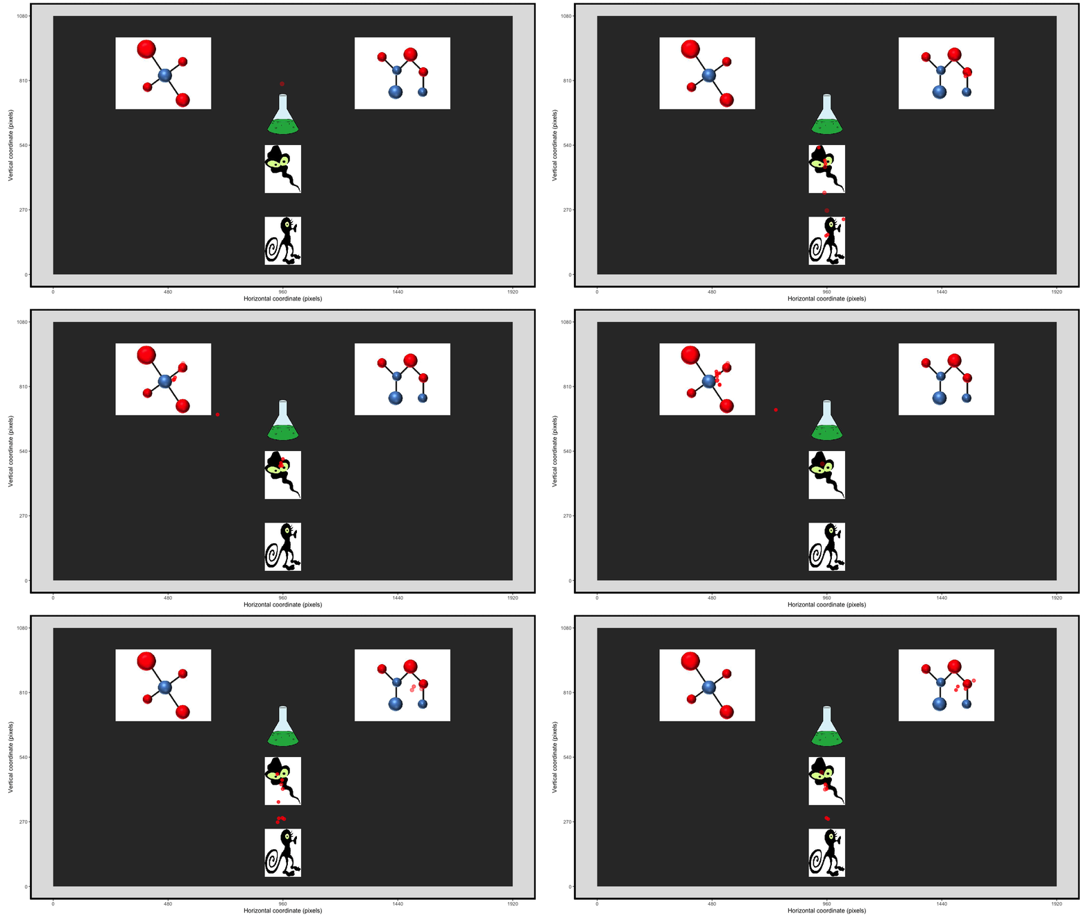
This animation takes raw data (of a single trial), transforms it into a larger dataset with plot-specific parameters, and then provides an animation of the participant’s gaze. The lag feature highlights the path taken and slowly fades to allow more data to be presented

data_plot1 <- data_smooth |> 
  filter(pNum == "118", trial == "1") |> # take a single participant and trial
  mutate(id = seq(1, n()), # add an ID column to original dataset,
         type = "original",
         size = 10, # specify initial size
         alpha = 1) |> # specify initial alpha
  mutate(time = time - min(time))

#bind the original dataset to a mid and end state too
data_plot1 <- rbind(data_plot1,
                data_plot1 |> # create second version of the dataset - this is the tail
                  mutate(type = "mid_state",      
                         time = time + 45,         
                         size = size * 0.5,        
                         alpha = alpha * 0.2),     
                
                data_plot1 |>                           
                  mutate(type = "end_state",      
                         time = time + 300, # this determines the length of the tail and the final state   
                         size = size * 0.5,        
                         alpha = 0))            

# pass this combined dataset to ggplot & animate
plot_animate <- data_plot1 |>
  ggplot(aes(x = x, y = y, group = id,
             size = size, alpha = alpha)) +
  # add a background image
  annotation_raster(magick::image_read("../data/HCL_sample_image.jpg"),
                    xmin = 0,
                    xmax = 1920,
                    ymin = 0,
                    ymax = 1080) +
  geom_point(colour = "red") +
  transition_components(time) +
  scale_size_identity() +
  scale_alpha_identity() +
  lims(x = c(0, 1920), y = c(0, 1080))

animate(plot_animate,
        duration =  round(max(data_plot1$time)/1000),
        start_pause = 5)

## To save an animation
#anim_save("figures/point_lag.gif", plot_animate, height = 1080, width = 1920, duration = round(max(data_plot1$time)/1000),
#          end_pause = 5)

Graphic showing the raw eye gaze data imposed over a sample stimuli image.

Plotting raw and smoothed data

We can also improve upon the static plot presented in the smoother() function by animating the x and y together.

data_both <- data |> 
  left_join(data_smooth, suffix = c("_raw", "_smooth"), by = join_by("pNum", "time", "trial")) |> 
    filter(pNum == "118", trial == "1") # take a single participant and trial

data_both <- data_both |> 
  pivot_longer(cols = c("x_raw", "x_smooth"), values_to = "x", names_to = "x_names") |> 
  pivot_longer(cols = c("y_raw", "y_smooth"), values_to = "y", names_to = "y_names") |> 
  filter((x_names == "x_raw" & y_names == "y_raw") | (x_names == "x_smooth" & y_names == "y_smooth")) |> 
  mutate(smoothed = str_remove(x_names, "x_"), .after = trial) |> 
  select(-c(x_names, y_names))

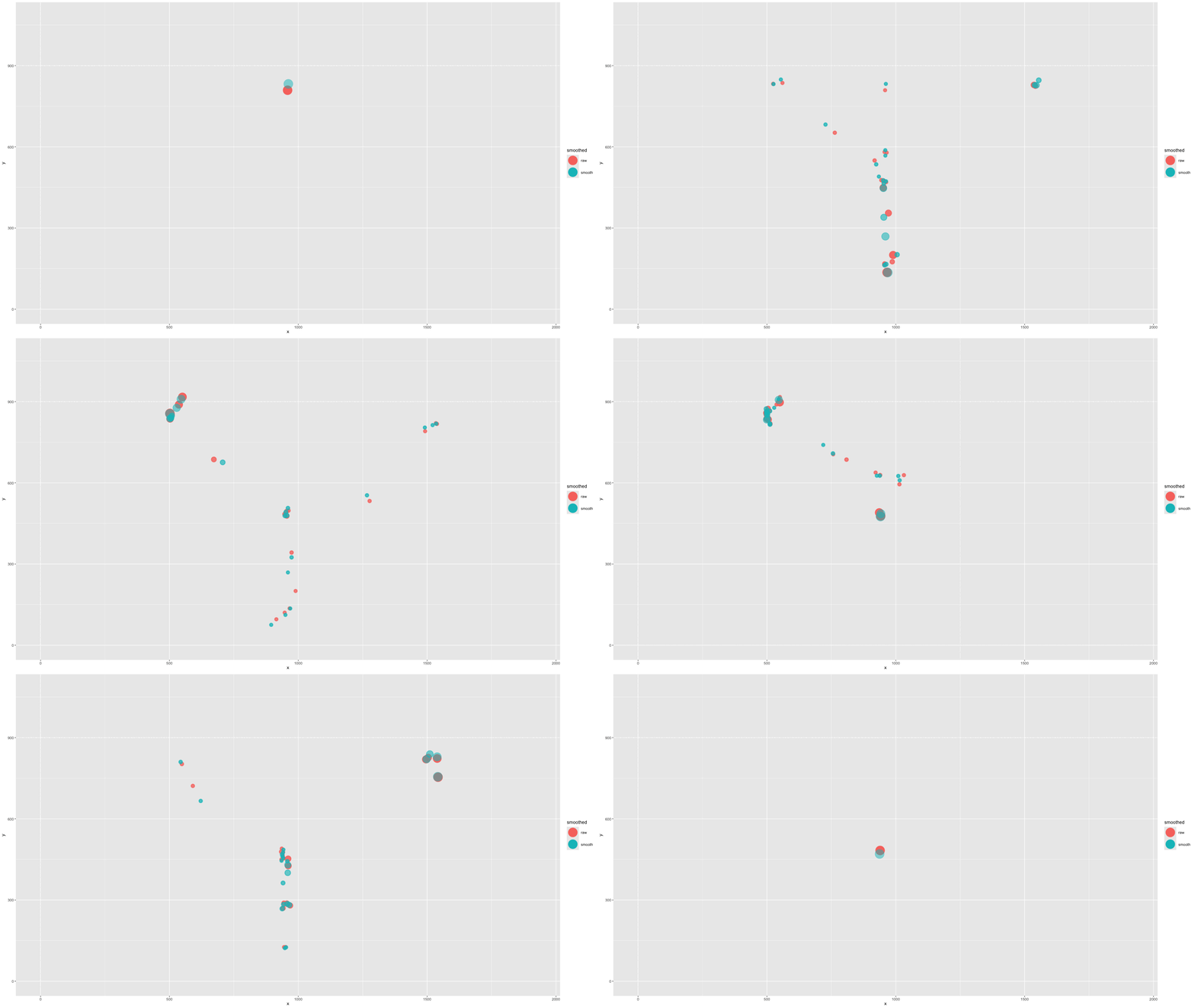
This first plot is quite rudimentary but shows a single timepoint position and the difference between the raw and smoother() data. The smoothed data is transparent to stop it from obscuring the raw data where they are well aligned.

plot_animate_smooth <- data_both |> 
  mutate(alpha = ifelse(smoothed == "smooth", .5, 1)) |> 
  ggplot(aes(x = x, y = y, colour = smoothed, fill = smoothed, alpha = alpha)) +
  geom_point(size = 10) +
  lims(x = c(0, 1920), y = c(0, 1080)) +
  scale_alpha_identity() +
  transition_components(time)

animate(plot_animate_smooth,
        duration =  round(max(data_both$time)/1000),
        start_pause = 5)

Image showing single timepoint difference between raw and smoothed data

Combining the smooth plot with the lag plot

A much more sophisticated plot is made by combining the lag plot and the smoother() comparison plot. In doing so, and tweaking some values, we can see how well the smoothed data adheres to the original data whilst removing the jerkiness of the raw data

data_plot3 <- data_both |>
  mutate(id = seq(1, n()), # add an ID column to original dataset,
         type = "original",
         size = 10, # specify initial size
         alpha = 1) |> # specify initial alpha
  mutate(time = time - min(time)) |> 
  arrange(time, desc(smoothed))

#bind the original dataset to a mid and end state too
data_plot3 <- rbind(data_plot3,
                data_plot3 |> # create second version of the dataset - this is the tail
                  mutate(type = "mid_state",      
                         time = time + 45,         
                         size = size * 0.5,        
                         alpha = 1),     
                
                data_plot3 |>                           
                  mutate(type = "end_state",      
                         time = time*2, # this determines the length of the tail and the final state   
                         size = size * 0.5,        
                         alpha = 1))            

data_plot3 <- data_plot3 |> 
  mutate(time = ifelse(time > max(data_both$time), max(data_both$time), time)) |> 
  mutate(alpha = ifelse(type %in% c("mid_state", "end_state") & smoothed == "smooth", .2, alpha))

# pass this combined dataset to ggplot & animate
plot_animate3 <- data_plot3 |>
  ggplot(aes(x = x, y = y, colour = smoothed, group = id,
             size = size, alpha = alpha)) +
  # add a background image
  #annotation_raster(magick::image_read("../data/HCL_sample_image.jpg"),
  #                  xmin = 0,
  #                  xmax = 1920,
  #                  ymin = 0,
  #                  ymax = 1080) +
  geom_point() +
  transition_components(time) +
  scale_size_identity() +
  scale_alpha_identity() +
  lims(x = c(0, 1920), y = c(0, 1080))

animate(plot_animate3,
        duration = round(max(data_plot3$time)/1000),
        start_pause = 5)

Image showing lagged timepoint difference between raw and smoothed data

Plotting AOI entries over raw data

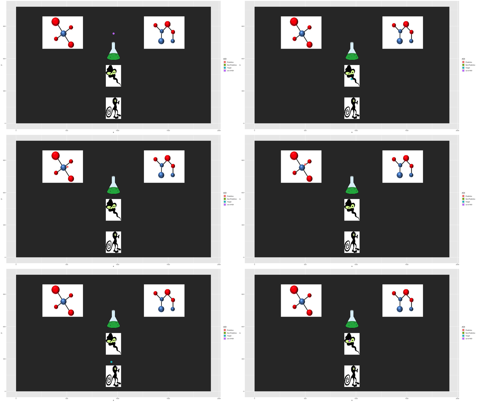
This section enables the plot colour to change when the eye is detected within an AOI.

data_plot4 <- data_smooth |> 
  filter(pNum == 118, trial == 1) |> 
  mutate(in_AOI = case_when(between(x, HCL_AOIs$x[1] - HCL_AOIs$width_radius[1]/2, HCL_AOIs$x[1] + HCL_AOIs$width_radius[1]/2) & 
                              between(y, HCL_AOIs$y[1] - HCL_AOIs$height[1]/2, HCL_AOIs$y[1] + HCL_AOIs$height[1]/2) ~ TRUE,
                            between(x, HCL_AOIs$x[2] - HCL_AOIs$width_radius[2]/2, HCL_AOIs$x[2] + HCL_AOIs$width_radius[2]/2) & 
                              between(y, HCL_AOIs$y[2] - HCL_AOIs$height[2]/2, HCL_AOIs$y[2] + HCL_AOIs$height[2]/2) ~ TRUE,
                            between(x, HCL_AOIs$x[3] - HCL_AOIs$width_radius[3]/2, HCL_AOIs$x[3] + HCL_AOIs$width_radius[3]/2) & 
                              between(y, HCL_AOIs$y[3] - HCL_AOIs$height[3]/2, HCL_AOIs$y[3] + HCL_AOIs$height[3]/2) ~ TRUE,
                            .default = FALSE)) |> 
    mutate(id = seq(1, n()), # add an ID column to original dataset,
         type = "original",
         size = 10, # specify initial size
         alpha = 1) |> # specify initial alpha
  mutate(time = time - min(time))



  x <- HCL_AOIs$x
  y <- HCL_AOIs$y
  width_radius <- HCL_AOIs$width_radius
  height <- HCL_AOIs$height
  rect_AOIs <- HCL_AOIs[!is.na(HCL_AOIs$height),]

plot_animate_4 <- data_plot4 |>
  ggplot(aes(x = x, y = y,
             colour = in_AOI
             )) +
  lims(x = c(0, 1920), y = c(0, 1080)) +
   #add a background image
   annotation_raster(magick::image_read("../data/HCL_sample_image.jpg"),
                  xmin = 0,
                  xmax = 1920,
                  ymin = 0,
                  ymax = 1080) +
  geom_point(aes(group = id))  +
      #geom_tile(data = rect_AOIs,
      #          aes(x = x, y = y, width = width_radius, height = height),
      #          colour = "dark blue",
      #          fill = "blue",
      #          alpha = .1) +
  transition_components(time)

animate(plot_animate_4, 
        duration = round(max(data_plot4$time)/1000))

Image showing lagged timepoint difference between raw and smoothed data

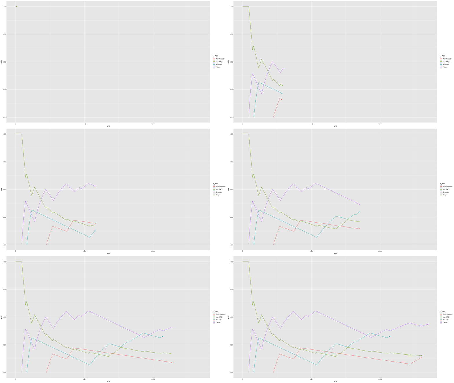
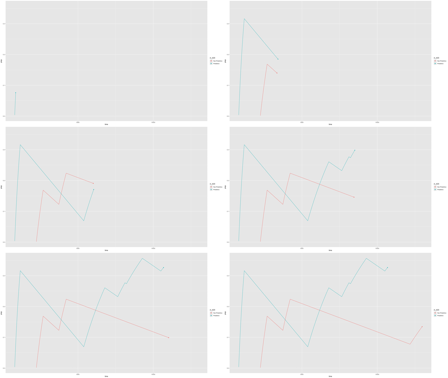
Plotting time spent in Areas of Interest over time

data_growth <- data_smooth |> 
  filter(pNum == 118, trial == 1) |> 
  mutate(in_AOI = case_when(between(x, HCL_AOIs$x[1] - HCL_AOIs$width_radius[1]/2, HCL_AOIs$x[1] + HCL_AOIs$width_radius[1]/2) & 
                              between(y, HCL_AOIs$y[1] - HCL_AOIs$height[1]/2, HCL_AOIs$y[1] + HCL_AOIs$height[1]/2) ~ "AOI_1",
                            between(x, HCL_AOIs$x[2] - HCL_AOIs$width_radius[2]/2, HCL_AOIs$x[2] + HCL_AOIs$width_radius[2]/2) & 
                              between(y, HCL_AOIs$y[2] - HCL_AOIs$height[2]/2, HCL_AOIs$y[2] + HCL_AOIs$height[2]/2) ~ "AOI_2",
                            between(x, HCL_AOIs$x[3] - HCL_AOIs$width_radius[3]/2, HCL_AOIs$x[3] + HCL_AOIs$width_radius[3]/2) & 
                              between(y, HCL_AOIs$y[3] - HCL_AOIs$height[3]/2, HCL_AOIs$y[3] + HCL_AOIs$height[3]/2) ~ "AOI_3",
                            .default = "none")) |> 
  select(-x, -y)


data_growth <- data_growth |> 
  #filter(in_AOI %in% c("AOI_1", "AOI_2")) |> 
  mutate(time_diff = c(0, diff(time))) |> 
  group_by(in_AOI) |> 
  mutate(time_diff = cumsum(time_diff)) |> 
  ungroup() |> 
  complete(pNum, time, trial, in_AOI) |> 
  group_by(in_AOI) |> 
  mutate(time_diff = ifelse(time == 0, 0, time_diff),
         time_diff = na.locf(time_diff,na.rm = FALSE)) |> 
  ungroup() |> 
  mutate(prop = time_diff/time)

####
growth_all <- data_growth |> 
  ggplot(aes(time, prop, colour = in_AOI, group = in_AOI)) +
  scale_colour_discrete() +
  geom_line() +
  geom_point() +
  transition_reveal(time)

animate(growth_all, 
        duration = round(max(data_growth$time)/1000))

Image showing the proportion of time spent in an AOI over time

Or just predictive and non-predictive cues

Done by adding a single filter in the in_AOI column

data_growth_partial <- data_smooth |> 
  filter(pNum == 118, trial == 1) |> 
  mutate(in_AOI = case_when(between(x, HCL_AOIs$x[1] - HCL_AOIs$width_radius[1]/2, HCL_AOIs$x[1] + HCL_AOIs$width_radius[1]/2) & 
                              between(y, HCL_AOIs$y[1] - HCL_AOIs$height[1]/2, HCL_AOIs$y[1] + HCL_AOIs$height[1]/2) ~ "AOI_1",
                            between(x, HCL_AOIs$x[2] - HCL_AOIs$width_radius[2]/2, HCL_AOIs$x[2] + HCL_AOIs$width_radius[2]/2) & 
                              between(y, HCL_AOIs$y[2] - HCL_AOIs$height[2]/2, HCL_AOIs$y[2] + HCL_AOIs$height[2]/2) ~ "AOI_2",
                            between(x, HCL_AOIs$x[3] - HCL_AOIs$width_radius[3]/2, HCL_AOIs$x[3] + HCL_AOIs$width_radius[3]/2) & 
                              between(y, HCL_AOIs$y[3] - HCL_AOIs$height[3]/2, HCL_AOIs$y[3] + HCL_AOIs$height[3]/2) ~ "AOI_3",
                            .default = "empty")) |> 
  select(-x, -y)


data_growth_partial <- data_growth_partial |> 
  filter(in_AOI %in% c("AOI_1", "AOI_2")) |> #only real difference
  mutate(time_diff = c(0, diff(time))) |> 
  group_by(in_AOI) |> 
  mutate(time_diff = cumsum(time_diff)) |> 
  ungroup() |> 
  complete(pNum, time, trial, in_AOI) |> 
  group_by(in_AOI) |> 
  mutate(time_diff = ifelse(time == 0, 0, time_diff),
         time_diff = na.locf(time_diff,na.rm = FALSE)) |> 
  ungroup() |> 
  mutate(prop = time_diff/time)

####
growth_partial <- data_growth_partial |> 
  ggplot(aes(time, prop, colour = in_AOI, group = in_AOI)) +
  scale_colour_discrete() +
  geom_line() +
  geom_point() +
  transition_reveal(time)

animate(growth_partial, 
        duration = round(max(data_growth$time)/1000))